What a Negative Result Is Worth

A search comes back empty. What have you learned? On its own, nothing — "we looked and found nothing" is a sentence about the dark and about the torch in equal measure, and without knowing the torch you cannot separate them. This is the second half of an arc whose first half ended with a concept falsified by its own kill condition. The machinery outlived the concept, and this is what we did with it: ran it where the right answer was nothing, then measured how faint a thing it would have missed, then watched one of our own written-down limits fall to a measurement we should have taken first.

The experiment where the right answer is nothing

The previous run had found a planted tone to the tenth of a hertz. That is impressive and it is not, by itself, evidence the method works — a machine that reports a tone wherever you point it will also be right whenever there is one.

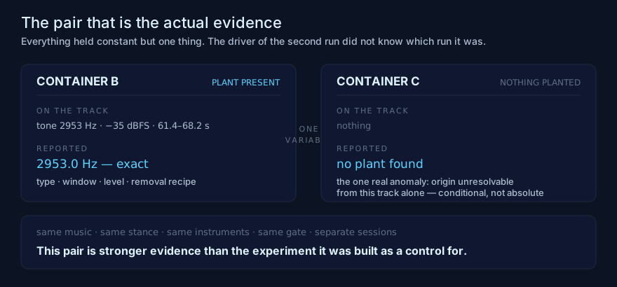
So: a third container, same music, same instruments, same task, and the same instruction to suspect a planted artefact. Nothing was planted.

The driver did not know that. The key was sealed, the preregistration was sealed, and — this is the part worth copying — the name of the experiment was sealed too. The working directory was named after the container’s identifier rather than its purpose, because the words “null test” would themselves have been the answer.

It reported no plant found.

And it did something better than that with the track’s one genuine anomaly, a seven-second sliding lowpass at the start. It said the origin cannot be resolved from this track alone: a moving edge rules out a fixed band cut, but a filter that is part of the composition and one added afterwards cannot be told apart without a clean reference. Conditional, not absolute. That is the honest verdict, and it is a harder thing to produce than either “clean” or “artefact”.

That pair is stronger evidence than the whole experiment in the previous part. Same music, same stance, same instruments, same gate, separate sessions, one variable: the plant. One found it to the hertz. The other did not invent one.

Two containers side by side. Container B had a tone planted at 2953 Hz, minus 35 dBFS, between 61.4 and 68.2 seconds, and reported 2953.0 Hz exactly plus the window, level, type and a removal recipe. Container C had nothing planted and reported no plant found, and said of the track's one real anomaly that its origin cannot be resolved from this track alone. Same music, same stance, same instruments, same gate, separate sessions, one variable. — The control is the evidence. One found it to the hertz; the other, given the same prompt to suspect a plant, did not invent one — and said so conditionally where the honest answer was conditional.

So we measured the torch

The null test proved the method does not invent. It said nothing about how faint a real thing could be before the method stopped seeing it — and until that number exists, “no plant found” means only “no plant found that we would have found”, which is circular.

So the same tone went into the same window of the same track six times, at descending levels from −35 down to −60 dBFS, and each meter was asked where it stopped reading.

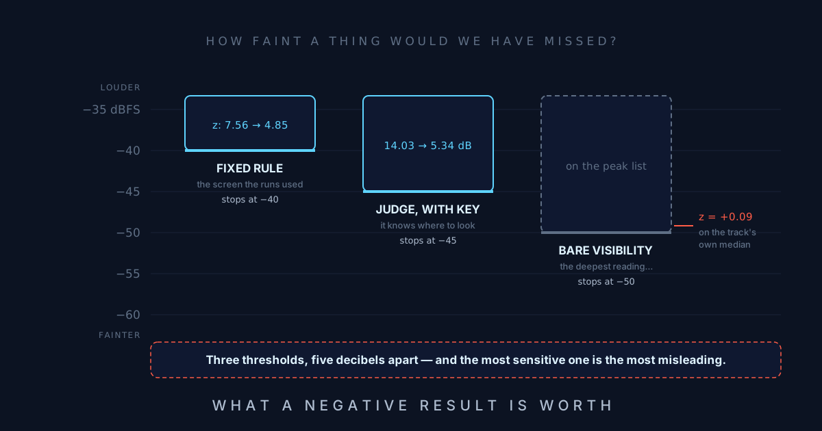
The answer is that there is no single threshold. There are three, and they are about five decibels apart.

level	on the peak list	z (fixed rule)	judge, with the key
−35 dBFS	yes	+7.56	14.03 dB
−40 dBFS	yes	+4.85	9.38 dB
−45 dBFS	yes	+2.35	5.34 dB
−50 dBFS	yes	+0.09	2.46 dB
−55 dBFS	no	—	0.94 dB
−60 dBFS	no	—	0.31 dB

The fixed mechanical rule — the screen the containers actually used to flag anomalies — breaks between −40 and −45 dBFS.

The judge holding the key breaks between −45 and −50, about five decibels deeper. That is expected rather than impressive: it knows which frequency to look at.

Bare visibility on the peak list survives to −50 and dies between −50 and −55. It is the most sensitive reading and the most misleading one, and the reason is in the table: at −50 dBFS the tone is on the list with z = +0.09 — sitting essentially exactly on the track’s own median prominence, among the music’s own peaks, indistinguishable from them. It is visible and it is not distinguishable, and those are different words.

So the earlier “no plant found” now has a sentence that means something: no local narrowband plant at or above about −40 dBFS, in this music, at this frequency. Not “the track is clean”. That version is true and the short version never was.

MATH BOX

A null with no floor is a likelihood ratio of one

The value of a negative result is bounded by the probability that the test would have found the thing had it been there. Write it as the ratio of the two likelihoods: how probable is “not found” if the artefact is present, against how probable it is if the artefact is absent. When the test cannot see an artefact of that size, both are close to one, the ratio is one, and the observation moves no belief at all. Reporting a null without its detection floor reports exactly that ratio and calls it evidence — which is the crisp version of the clinical rule that absence of evidence is not evidence of absence (Altman & Bland, BMJ 1995), and the reason statistical power is a property you are supposed to state before you interpret a null (Cohen, 1988). The detection floor is the effect size at which power becomes usable; it is not an optional extra, it is the null’s units.

Two features of this instrument make the point sharper than the textbook version.

The floor is a property of the material, not of the instrument alone. The threshold is computed from the track’s own distribution — the median and the median absolute deviation of prominences across its windows — so a spectrally denser piece of music raises its own bar. Power here is not a constant you measure once. It travels with the sample.

And the contaminant moves the scale it is judged against. A flat, track-length artefact adds high values to that distribution. The median barely notices, exactly as robust-statistics theory says it should not — the median’s breakdown point is 50 %, so a contaminant occupying at most a third of the pool cannot shift it (Hampel, 1971). The scale estimate has no such immunity in this direction: our measured MAD went from 1.66 to as much as 3.47 dB, and since the rule fires at k · MAD, the artefact raises the bar it has to clear. That is why the firing count is not monotone in level — at −45 dBFS the tone tripped the rule in one window and at −50 dBFS in two.

The limit that lived two hours

Yesterday morning a mapping session wrote a hard limit into the project’s living document: the mechanical rule is structurally blind to a flat, track-length artefact, because the median and the deviation come from the track’s own windows and something present in every window cannot stand out from them. A product option was closed on the strength of it.

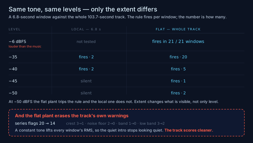
It was an argument. It had never been run. So it was run — same tone, same track, same grid, one variable: the artefact’s extent, a 6.8-second window against the whole 103.7 seconds.

The rule fires at every level tested, from −6 down to −50 dBFS. Including −50, where the local plant at the same level does not fire it at all.

And the decisive row is the loud one. At −6 dBFS the planted tone is louder than the entire piece of music — the track peaks at −9.70 dBFS — and a structurally blind rule would not see that either. It fired in all twenty-one windows.

The reasoning had picked the wrong channel. The prominence rule pools the top three peaks from every window into one distribution, so a flat tone occupies at most a third of it and the median holds: 9.26 → 10.36 dB. What moves is the spread, and that is the mechanism from the box above.

What survives is worse than the claim it replaced. The series rules — band energy, crest factor, noise floor — are genuinely blind to a flat artefact, one value per window and all of them shifted equally. But they do not merely fall silent. The flat plant erased six of the track’s own twenty anomaly flags: a constant tone lifts the RMS in every window, so the crest factor compresses, the noise-floor estimate rises, and the track’s quiet intro stops looking quiet.

A flat artefact makes the track score cleaner.

And there is one more thing in the same report, which is the part that would keep me up. The prominence rule flags the tone as an anomaly. The persistence rule — which classifies a frequency present in most windows as the track’s own material — lists the same tone, at every level from −6 to −50, as belonging to the music. Two rules, one report, opposite answers, and each one alone reads as confident.

NERD BOX

Blinding, and the bookkeeping slip that nearly falsified everything

Blinding a null test is harder than blinding a normal one, because the existence of the test is informative. The key was sealed, the preregistration was sealed, and the working directory was named by the container’s identifier — “null test” as a folder name would have been the answer written on the envelope. Four preregistered predictions, all four hit: no false find, a gate total of 20 against a predicted 16 in an 8-to-26 interval, no anomalies after the 23-second mark on either grid, and an explicit verdict rather than a hedge.

And a slip worth publishing. That container’s driver ran the gate correctly — twenty positive verdicts by three-vote majority, none unreadable — and then failed to record the state transition. Counted mechanically from the database, its score would have read zero instead of twenty.

The same forgetting in either of the two earlier containers would have falsified the whole concept from a bookkeeping error, because the ratio in the previous part was computed from exactly that field. A metric that measures performance depended on whether the driver remembered to write it down — which is the metric’s fault and not the driver’s, and it is the same lesson as the previous part arriving from a different direction. Fixed in both directions: that container’s states were recovered from the stored verdicts rather than guessed, and gate results are now written by a single command.

The same tone at the same levels, planted locally in a 6.8 second window against flatly across the whole track. Local fires in two windows at minus 35 and minus 40 and is silent at minus 45 and minus 50. Flat fires in twenty-one windows at minus 6, twenty at minus 35, five at minus 40, one at minus 45 and two at minus 50. Footer: the flat plant erased six of the track's own twenty anomaly flags, so the track scores cleaner. — At −50 dBFS the flat plant trips the rule and the local one does not. And the footer is the part that matters: the same artefact quietly removes six of the track's own warnings.

The correction we owed about ourselves

The level sweep had been run by a script written for the occasion and left in a temporary directory. Writing it down properly as a permanent tool was housekeeping, and it caught something.

Validated against the published result before being used, the harness reproduced the planted files bit for bit and the prominences and judge readings exactly — and did not reproduce the z column. The comparison distribution the published table reported (median 10.18, MAD 1.54) matches none of the measured tracks; the rule gives 9.27 / 1.78.

All three thresholds survive, because they depend on which side of the line a value falls rather than how far. One claim does not: −50 dBFS is not below the track’s median, it is essentially on it. z = +0.09, not −0.63.

The point that visibility is not distinguishability comes out stronger from the corrected number — z ≈ 0 is the purest possible statement of “indistinguishable” — and the published number was still wrong. Both of those are true at once, and the second one is the one that gets fixed in public.

The one-off script in a temporary directory is why it went out unchecked. That is the whole finding.

What survives

A null result’s unit is its detection floor. Without one, “we found nothing” is not a weak result, it is not a result — it is a statement whose two possible causes it cannot distinguish.
Blind the name, not just the answer. When the existence of a test is informative, the folder name is part of the blinding.
There is no single sensitivity. Ours had three thresholds five decibels apart, and the most sensitive of them was the most misleading — visible is not distinguishable.
Sensitivity depends on extent, not only on level. A local artefact and a flat one at the same level are seen by different rules, in opposite ways, and by one of them not at all.
A limit written down from an argument is a claim, not a finding — and decisions get made on it in the meantime. Ours lived two hours and closed an option while it did.
A meter that reads all clear because of the fault is worse than one that goes quiet. Whatever else this instrument gets used for, that one is going in the specification.

The concept that built all this was falsified. The instruments were not — they were null-tested, calibrated, and used to overturn one of our own conclusions inside a day, which is a better retirement than most ideas get.

Sources & further reading

D.G. Altman & J.M. Bland, Absence of evidence is not evidence of absence (BMJ, 1995) — the one-page statement of why a null needs its power before it can be read.
J. Cohen, Statistical Power Analysis for the Behavioral Sciences (2nd ed., 1988) — power as a property you declare in advance, and effect size as the unit a null is measured in.
F.R. Hampel, A General Qualitative Definition of Robustness (Annals of Mathematical Statistics, 1971) — the breakdown point, and why the median held while the scale estimate did not.
P.J. Rousseeuw & C. Croux, Alternatives to the Median Absolute Deviation (JASA, 1993) — the MAD’s behaviour as a scale estimate, and what it is and is not immune to.
I.J. Good, Weight of Evidence: A Brief Survey (1985) — the likelihood-ratio framing of what an observation is worth.
B.A. Nosek et al., The preregistration revolution (PNAS, 2018) — including the four predictions this null test was scored against.

— SF3D